Miasm IR getting higher
The Miasm intermediate representation is used for multiple task: emulation through its jitter engine, symbolic execution, DSE, program analysis, … But the intermediate representation can be a bit hard to read. We will present in this article new tricks Miasm has learnt in 2018. Among them, the SSA/Out-of-SSA transformation, expression propagation and high level operators which can be joined to “lift” Miasm IR to a more human readable language.
This article is based on Miasm version v0.1.1.
Note: We use graphviz to illustrate some graphs. Its layout does not always totally conform with a reverse engineering “ideal view”, so please be tolerant with those odd graphs.
Problem
As we saw in the Release v0.1.0 article, the traduction from native language to Miasm intermediate representation can be quite verbose. For the simple x86 code:
cmp     eax, ebx
jg      XXX
The resulting IR was:
af = ((EAX ^ EBX) ^ (EAX + -EBX))[4:5]
pf = parity((EAX + -EBX) & 0xFF)
zf = (EAX + -EBX)?(0x0,0x1)
of = ((EAX ^ (EAX + -EBX)) & (EAX ^ EBX))[31:32]
nf = (EAX + -EBX)[31:32]
cf = (((EAX ^ EBX) ^ (EAX + -EBX)) ^ ((EAX ^ (EAX + -EBX)) & (EAX ^ EBX)))[31:32]

EIP = (zf | (nf + -of))?(loc_key_41,loc_key_40)
IRDst = (zf | (nf + -of))?(loc_key_41,loc_key_40)
Here, each flag (from the cmp instruction) has a computable equation, mainly based on known bit hacks.
The problem is that using this representation, it is hard to answer simple questions like:
- which arguments are tested by the condition?
- which kind of condition is it?
Another point which worsen the problem is the simplification engine. Indeed, we planned to use this engine to keep the possibility to later transform these expressions into corresponding comparisons (miasm2/expression/simplifications_cond.py).
Unfortunately, if the instructions were:
cmp     eax, 0x10
jg      XXX
The resulting IR was:
af = ((EAX ^ 0x10) ^ (EAX + -0x10))[4:5]
pf = parity((EAX + -0x10) & 0xFF)
zf = (EAX + -0x10)?(0x0,0x1)
of = ((EAX ^ (EAX + -0x10)) & (EAX ^ 0x10))[31:32]
nf = (EAX + -0x10)[31:32]
cf = (((EAX ^ 0x10) ^ (EAX + -0x10)) ^ ((EAX ^ (EAX + -0x10)) & (EAX ^ 0x10)))[31:32]

EIP = (zf | (nf + -of))?(loc_key_41,loc_key_40)
IRDst = (zf | (nf + -of))?(loc_key_41,loc_key_40)
After a pass of expression simplification, this code became:
af = (EAX ^ (EAX + 0xFFFFFFF0) ^ 0x10)[4:5]
pf = parity((EAX + 0xFFFFFFF0) & 0xFF)
zf = (EAX + 0xFFFFFFF0)?(0x0,0x1)
of = ((EAX ^ (EAX + 0xFFFFFFF0)) & (EAX ^ 0x10))[31:32]
nf = (EAX + 0xFFFFFFF0)[31:32]
cf = (EAX ^ ((EAX ^ (EAX + 0xFFFFFFF0)) & (EAX ^ 0x10)) ^ (EAX + 0xFFFFFFF0) ^ 0x10)[31:32]

EIP = (zf | (nf + -of))?(loc_key_41,loc_key_40)
IRDst = (zf | (nf + -of))?(loc_key_41,loc_key_40)
Here, the condition is even harder to extract: we may have to recognize that the constant 0xFFFFFFF0 is in fact -0x10 to get back the original operands (look at the constants to match in the cf equation).
To avoid this information loss, the idea is the introduction of intermediate operators standing for actual flag equations.
Hence, we decided to rewrite key mnemonics of each architecture semantic in order to generate the following IR:
af = ((EAX ^ EBX) ^ (EAX + -EBX))[4:5]
pf = parity((EAX + -EBX) & 0xFF)
zf = FLAG_EQ_CMP(EAX, EBX)
of = FLAG_SUB_OF(EAX, EBX)
nf = FLAG_SIGN_SUB(EAX, EBX)
cf = FLAG_SUB_CF(EAX, EBX)

EIP = CC_S>(nf, of, zf)?(loc_key_40,loc_key_41)
IRDst = CC_S>(nf, of, zf)?(loc_key_40,loc_key_41)
Note we have inserted another special high level operator here in the jump condition: the CC_S> operator. It’s the same mechanism as the FLAG_XXX. Instead of taking the explicit computation between flags, it will simply take them as parameters. Thus, no more reductions or interference will affect them.
The trick is that even in the case of the constant operator, the intermediate representation will be a bit more coherent (assume we ignore the af and pf flags here):
af = (EAX ^ (EAX + 0xFFFFFFF0) ^ 0x10)[4:5]
pf = parity((EAX + 0xFFFFFFF0) & 0xFF)
zf = FLAG_EQ_CMP(EAX, 0x10)
of = FLAG_SUB_OF(EAX, 0x10)
nf = FLAG_SIGN_SUB(EAX, 0x10)
cf = FLAG_SUB_CF(EAX, 0x10)

EIP = CC_S>(nf, of, zf)?(loc_key_40,loc_key_41)
IRDst = CC_S>(nf, of, zf)?(loc_key_40,loc_key_41)
If a simplification happens in one argument of the FLAG_XXX operator, it must happen in other FLAG_YYY operands. Thus, each flag zf, of, nf, cf will be computed with identical sources. The next step is to make a match between the tested flags and the flags equations themselves in order to get back the correct high level operator used in the jump condition.
As stated in the previous article, we have special reduction rules which will reduce:
IRDst = CC_S>(
    FLAG_SIGN_SUB(EAX, EBX),
    FLAG_SUB_OF(EAX, EBX),
    FLAG_EQ_CMP(EAX, EBX)
    )?(loc_key_40,loc_key_41)
into:
IRDst = (EBX <s EAX)?(loc_key_40,loc_key_41)
As a result, information on the comparison has been kept in the IR.
But to do so, one needs to expand the zf, of, … sources in the CC_S> arguments. In the example given above, it’s quite immediate: there is no instructions and no flow which can interfere with those flags before the CC_S> operator, so we can “propagate” the flags values in the CC_S>. But it’s not always as simple. The more general question is “if EAX comes from another register, for example ECX, can I replace EAX in the CC_S> by ECX as well?”
To answer this question, we will use the SSA transformation in combination with the expression propagation.
SSA transformation
The SSA transformation won’t be fully explained here. You can find details here. The first important thing to know is that a register can only be affected once in the whole program. That is why you have different “versions” of a same register in SSA form (indexed with a number). The second important point is the way to represent the merging of different “possible” values in a control flow graph branch meeting: it’s solved using a special operator called Phi which takes different possible values issued in parent branches and stores the result in a new variable at the branches meeting.
Thanks to Tim Blazytko and Niko Schmidt, Miasm implements this transformation. Let’s work on the following code. It’s an arbitrary simple code which only focuses on the previous problem. More realistic examples are showcased at the end of the article, as well as an IDA plugin, which you can test on your own binaries!
int test_u32_greater(uint32_t a, uint32_t b)
{
    if (a > b)
        return 1;
    return 0;
}
First of all, here is the resulting intermediate representation using high level flags. To manipulate minimalist graphs, the dead_simp pass has been applied on the intermediate representation. It removes lines assigning unused registers.

Intermediate representation
Here is the resulting intermediate representation after the SSA pass:

SSA form
Note: the last two assignments, EAX.2 = EAX.1 and ESP.3 = ESP.2 are the result of side effects added before the SSA transformation in order to be able to track living registers after the end of the function: they represent the final value of their equivalent original registers EAX and ESP. The choice of which registers are important is not done in the SSA algorithm itself, but in the user code: it’s up to you to describe your ABI conventions.
In Miasm intermediate representation, registers never alias. For example the register AL does not exist: it’s represented as a slice of EAX. So in this graph, it’s easy to guess where does the zf.0 register used in the jump condition (IRDst) comes from. Note the information can also be retrieved on the original graph using the def/use chain algorithm (also implemented in Miasm, see DiGraphDefUse for more detail).
But an important point is that here, in SSA, the “propagation” of the zf.0 in the equation IRDst = CC_U<=(cf.0, zf.0)?(loc_8049276,loc_804926f) won’t interfere with any other zf register in the graph, as each zf has its own version.
Expression propagation
But that does not mean the replacement is as trivial as it seems. There are rules to check. In our case, the zf.0 comes from FLAG_EQ_CMP(EAX.0, @32[EBP.0 + 0xC]). So if we replace the zf.0 elsewhere by it’s original value, we have to verify that this original value is still valid at this point.
In this example, we have to be sure that @32[EBP.0 + 0xC] is not modified between the zf.0 definition, and the zf.0 use. Those rules are very similar to rules that can be involved in the compilation domain.
Here are some rules:
- do not propagate registers which depend on memory if there are memory writes between the register definition and register usage
- do not propagate registers which depend on call_func operators. Those operators are here to simulate sub calls.
- do not propagate registers coming from a Phi operator
These rules are not optimal, and sometimes correct propagations are missed. But it avoids more complex algorithm (requiring, for instance, “may-alias” analysis).
With this in mind, the propagation algorithm can work on the previous graph and propagate some registers values, for example zf.0, cf.0. The IRDst equation becomes:
IRDst = CC_U<=(
    cf.0 = FLAG_SUB_CF(EAX.0, @32[EBP.0 + 0xC]),
    zf.0 = FLAG_EQ_CMP(EAX.0, @32[EBP.0 + 0xC])
    )?(loc_8049276,loc_804926f)
As previously described, we have special reduction rules for those “high level” operators. So, the final graph is:

SSA after propagation
Note that Miasm makes the difference between signed comparisons represented using the operators <s or <=s, and unsigned comparisons represented using <u and <=u.
Out-of-SSA
The remaining operation is to jump back into a “classic world” by removing Phi operators. To do this, we have implemented the algorithm described in Revisiting Out-of-SSA Translation for Correctness, Code Quality, and Efficiency. To summarize, it exists a simple algorithm of Out-of-SSA transformation, but it will generate a lot of variable copies. This paper gives a quite interesting algorithm which does this effectively using very few variable copies. The result is the following graph:

After Out-of-SSA
What is interesting is that these algorithms work on the intermediate representation of Miasm. Thus, any supported Miasm architecture will give an equivalent result. Let’s check on aarch64:
- class center
- |aarch64_cfg| |aarch64_final|
On msp430 (take care, the destination is on the right hand):


Another one on mips32:


Let look at optimized version of the code, in mips32:


Let look at optimized version of the code, in arm:


This last graph needs some explanations: if we look closer at the conditional jumps, we can note that both conditions are identical, but destination are permuted. There are only two possible paths (not four), which result in R0.1 value set to 0 or 1.
Note that we could have a transformation which merge those two if/then pattern in only one if/then/else test (à la LLVM). We may re-implement each LLVM passes here! That’s why we are also working on another pass which can translate Miasm intermediate representation into LLVM-IR language. You can find a starting point of this here.
Note you can get those results using the Miasm plugin for IDA:
Final IR arm IDA
Note: sadly, we didn’t find a way to change the color of the edges in IDA GraphViewer API, that’s why every edges are blue. If you know a way to change this, don’t hesitate to open an issue or make a pull request in Miasm!
Stack analysis
For now, we only focused on registers propagation. It would be interesting to do this for stack variables as well. But here starts the troubles: the first hypothesis we used, “there are no alias on registers”, doesn’t stand for stack variables: they are in general stored in memory, and memory can alias. Resolving aliases is a known hard problem.
But our “propagated” version of the intermediate representation has special properties now. Looking at the stack accesses, we can note there is no more stack pointer aliases (from a register point of view): no more EBP, as it has been replaced by the equation depending on original value of ESP.
So we can do an attempt to “guess” how many local variables are present, and what are their sizes. To do this, a naive approach is to gather each memory lookup/write done through on an expression based on ESP. Once it’s done, we can create fake registers, using their corresponding variables sizes, and replace memory accesses by those registers.
This mechanism has been used in IDA decompiler, but may not be a as good idea as it seems. M. Guilfanov gives some interesting points on Hex-rays decompiler here: Guilfanov Decompiler Internals Microcode.
This mechanism is prone to alias errors: if you give the address of a local variable in a sub function call, the sub function will be able to change the content of your local variable and the propagation algorithm will be tricked.
Anyway, let’s take a simple example to illustrate it:
int func(unsigned char* s)
{
    int i;
    unsigned int sum = 0;

    for (i = 0; i < 10; i++) {
        sum += s[i];
    }
    return sum;
}
Here is the control flow graph:

Original CFG
Here is the propagated version:

Final unssa
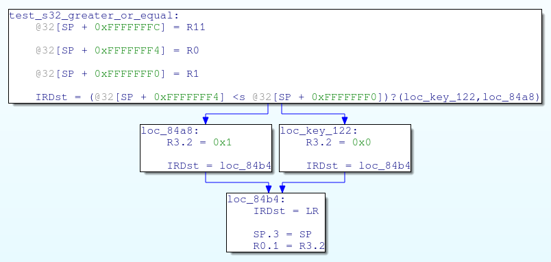
Here, the algorithm will recognize @32[ESP + 0xFFFFFFF4], @32[ESP + 0xFFFFFFF8], @32[ESP + 0xFFFFFFFC], @32[ESP], @32[ESP + 0x4] and @32[ESP + 0x8] as stack accessors. But only @32[ESP + 0xFFFFFFF4], @32[ESP + 0xFFFFFFF8], @32[ESP + 0xFFFFFFFC] will be marked as local stack, as accesses are done above the initial ESP value. Only them will be replaced by equivalent “register variables”. So the final graph will be:

Final unssa
If we recognize the index, the argument and the sum, we can rename those variables and get the final graph:

Final unssa
Examples
As promised, here are some examples. The first one is taken from an armthumb binary. First, the original control flow graph:

Function at 0x398
Then, the result obtained with (-p and -x are respectivly “generate the SSA form” and “do expression propagation”):
python2 miasm/example/disasm/full.py -m armtl firmware.bin 0x3B8 -p -x

Final result for 0x398
Then, another function:

Cfg of 0x576
Here we can observe the binary loads constants from static memory. We can ask full.py to effectively replace those memory accesses by their real values. Take care, this option is a bit dummy for now: for a classic ELF or PE, this must be done only from read only section but this is not the case for now. The script will read the memory value as soon as the memory address is a pure integer and its memory variable can be read from the source. Here is the final CFG:

Final analysis of 0x576
Conclusion
Don’t be tricked here: we are not doing decompilation. All this work may be a good start to enhance the intermediate representation output. As we saw, the final form is quite identical from one architecture to another, which is one goal of this intermediate representation. This representation can already be translated into LLVM as well, so this may be an interesting bridge to combine analysis. Another point is that the final form is quite easy to manipulate and understandable… Ok, maybe it’s up to you to judge! Anyway, transformations like SSA now opens a door to loop analysis, value analysis, types propagation/discovery and more!